This appendix documents the datasets used in this book. For each one: where it came from, what we did to it, and how to cite it.
The Meuse Dataset
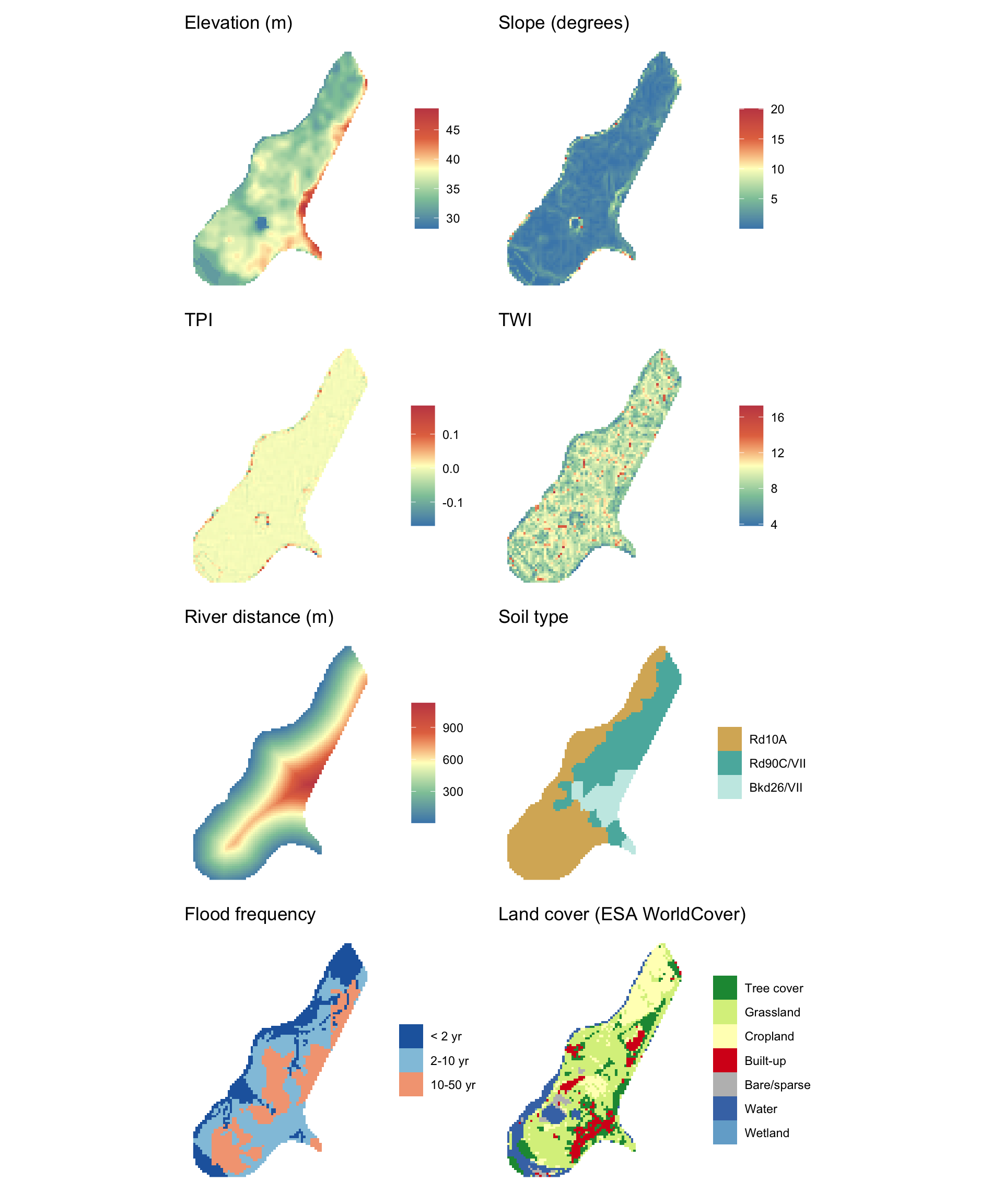
We use the Meuse River dataset throughout the geostatistics chapters. The original meuse.all from the gstat package has 17 columns, most of which we never touch - landuse codes, indicator variables for which survey the row came from, a lime field test result. Handing students a 17-column data frame when you only ever use 7 of those columns is a tax on attention. Same problem with the original meuse.grid: it had a normalized distance column and two arbitrary area-split columns (part.a, part.b) that served no purpose in this book. So we stripped both down. meuse2 has the coordinates and the metals plus organic matter. meuse.grid2 has the grid coordinates and a set of modern, interpretable covariates. The covariates that matter for the regression kriging chapter - soil type, flooding frequency, river distance - live in meuse.grid2 and get extracted onto the point data when needed using terra::extract(). That workflow is more realistic than having covariates pre-joined into the point dataset anyway.
Origin
The original data were collected in the early 1990s near the village of Stein in the Netherlands, in the floodplain of the Meuse River. The data include topsoil heavy metal concentrations (cadmium, copper, lead, zinc) at 155 sample locations, along with a handful of environmental covariates. The dataset was published and distributed with the sp package in R by Edzer Pebesma and Roger Bivand, and it has been a workhorse teaching dataset in spatial statistics ever since.
The original dataset comes in two objects from the sp package: meuse (155 sample points) and meuse.grid (the prediction grid). In this book we use trimmed versions of both. For the point data we use meuse2, and for the prediction grid we use meuse.grid2. Load them like this:
meuse.grid2 extends the original meuse.grid with modern covariate layers pulled from open data sources. Here is what was added and where it came from.
Elevation and terrain derivatives were pulled using the elevatr package (Hollister et al. 2025), which fetches AWS terrain tiles at roughly 10 m resolution (zoom level 14). The elevation raster was reprojected to RD New (EPSG:28992) before computing terrain derivatives with terra::terrain() and terra::flowAccumulation()(Hijmans 2026).
Land cover is from ESA WorldCover 2021, a global 10 m land cover product based on Sentinel-1 and Sentinel-2 imagery. The data are freely available from the ESA public S3 bucket and were accessed using the rstac package (Simoes et al. 2021). The study area straddles the boundary between two 3x3 degree tiles (N48E003 and N51E003), which were merged before cropping.
River distance was computed using main channel geometries pulled from OpenStreetMap via the osmdata package (Mark Padgham et al. 2017), filtered to features tagged as waterway=river with names matching Maas, Meuse, or Afgesneden Maas. Streams and canals were excluded to avoid spurious near-zero distances in the upland parts of the study area. Distance from each grid cell to the nearest retained feature was calculated in meters using sf::st_distance()(Pebesma 2026).
Fourteen boundary cells with NA terrain values (edge effects from the neighborhood calculations in terrain()) were dropped, leaving 3089 grid cells.
The script that builds the augmented grid is in rScripts/buildMeuseCovariates.R.
Variable descriptions
meuse2 (point data, 164 rows)
Variable
Units
Description
x
meters
Easting, RD New (EPSG:28992)
y
meters
Northing, RD New (EPSG:28992)
cadmium
mg/kg
Topsoil cadmium concentration
copper
mg/kg
Topsoil copper concentration
lead
mg/kg
Topsoil lead concentration
zinc
mg/kg
Topsoil zinc concentration
om
%
Topsoil organic matter
Note that meuse.all from gstat has 164 observations, nine more than the 155 in sp::meuse. The column in.meuse155 in the original flags which rows belong to the classic 155-point dataset. We keep all 164 in meuse2.
meuse.grid2 (prediction grid, 3089 rows)
Variable
Type
Description
x
numeric
Easting, RD New (EPSG:28992), meters
y
numeric
Northing, RD New (EPSG:28992), meters
soil
factor
Soil type (see below)
ffreq
factor
Flooding frequency class (see below)
elev_m
numeric
Elevation above sea level, meters
slope_deg
numeric
Terrain slope, degrees
aspect_deg
numeric
Aspect (direction of slope), degrees from north
tpi
numeric
Topographic position index: positive values are ridges/hilltops, negative values are valleys
twi
numeric
Topographic wetness index: higher values indicate areas where water accumulates
Non-calcareous weakly-developed meadow soils, heavy sandy clay to light clay
3
Bkd26/VII
Red Brick soil, fine-sandy, silty light clay
A note from the original documentation: it is questionable whether the soil data in meuse.grid2 come from a real soil map, as they do not match the published 1:50,000 map. Use them with that caveat in mind.
Flooding frequency (ffreq):
Code
Description
1
Once in two years
2
Once in ten years
3
Once in 50 years
The original documentation notes that it is not known how the flooding frequency map was generated.
ESA WorldCover land cover (landcover):
Code
Class
10
Tree cover
20
Shrubland
30
Grassland
40
Cropland
50
Built-up
60
Bare / sparse vegetation
80
Permanent water bodies
90
Herbaceous wetland
The full WorldCover legend has a few additional classes (snow/ice, mangroves, moss/lichen) that don’t appear in this area.
The file birdRichnessMexico.rds contains 200 point locations across Mexico, each with a count of bird species (nSpecies) plus a set of WorldClim bioclimatic variables.
Origin
The richness values come from the global bird species richness maps at BiodiversityMapping.org1, assembled by Clinton Jenkins at Florida International University. The maps are derived from BirdLife International v7 range maps (2018), processed at 10x10 km resolution in the Eckert IV equal-area projection, native extant species only.
We sampled 500 random points across Mexico from the richness raster, then subsampled to 200 for the exercises. The points were reprojected to North America Albers Equal Area Conic centered on Mexico (SR-ORG:38), giving coordinates in kilometers.
WorldClim variables
Six bioclimatic variables from WorldClim v2.1 (Fick and Hijmans 2017) at 10 arc-minute resolution were extracted to the point locations using the geodata and terra packages:
Variable
WorldClim code
Description
Units
mat
BIO1
Annual mean temperature
°C
tempSeason
BIO4
Temperature seasonality
SD × 100
tempRange
BIO7
Temperature annual range
°C
map
BIO12
Annual precipitation
mm
precipSeason
BIO15
Precipitation seasonality
CV
precipDryQ
BIO17
Precipitation of driest quarter
mm
The script that builds the dataset is in data/buildBirdRichnessMexico.R.
Permissions and citation
BiodiversityMapping.org permits free use for personal, not-for-profit purposes by students and educational institutions, with attribution. Cite the underlying papers when using the data:
Jenkins CN, Pimm SL, Joppa LN (2013). Global patterns of terrestrial vertebrate diversity and conservation. PNAS 110(28). doi:10.1073/pnas.1302251110
Pimm SL, Jenkins CN, Abell R, Brooks TM, Gittleman JL, Joppa LN, Raven PH, Roberts CM, Sexton JO (2014). The biodiversity of species and their rates of extinction, distribution, and protection. Science 344(6187): 1246752.
California Ozone and Precipitation
Two California datasets appear in the spatial data crash course and the interpolation chapters: ozone monitoring station records and weather station precipitation records. Both come from the rspat package by Robert Hijmans, which bundles teaching datasets for the rspatial.org tutorials.
California ozone (californiaOzonePoints.csv)
345 ozone monitoring stations across California with mean daily ozone (parts per billion, averaged 1980-2009). Originally from the US EPA Air Quality System. In rspat this is the airqual dataset; we exported it to CSV and trimmed to three columns (ozone, longitude, latitude). Used in the spatial data crash course to demonstrate point data and raster extraction.
California precipitation (prcpCA.rds, gridCA.rds)
prcpCA.rds has 432 weather stations with monthly and annual precipitation totals (mm), station names, elevations, and coordinates in the California Teale Albers projection (EPSG:3310). Station IDs follow the rspat convention (e.g., ID741 = Death Valley). In rspat this is the precipitation dataset.
gridCA.rds is a 4053-point regular prediction grid covering California in the same projection, used as the interpolation target in the IDW and kriging exercises.
Citation
Both datasets are distributed with the rspat package and should be cited as:
Hijmans RJ (2023). rspat: rspatial.org data. R package. https://github.com/rspatial/rspat
Image Credits
The three mushroom photographs in the Point Patterns chapter come from Wikimedia Commons and are reused under Creative Commons licenses, with attribution as required. A machine-readable log of these credits, suitable for a publisher’s permissions desk, lives in permissions.csv at the repository root.
The Hebeloma image is licensed under CC BY-SA 3.0 (ShareAlike): it is reused as-is, and any adaptation of that photo would have to carry the same license. The Lactarius pubescens image is dual-licensed under GFDL 1.2+ and CC BY 3.0; it is used here under CC BY 3.0.
Fick, Stephen E., and Robert J. Hijmans. 2017. “WorldClim 2: New 1-Km Spatial Resolution Climate Surfaces for Global Land Areas.”International Journal of Climatology 37 (12): 4302–15. https://doi.org/10.1002/joc.5086.
Hollister, Jeffrey, Tarak Shah, Jakub Nowosad, Alec L. Robitaille, Marcus W. Beck, and Mike Johnson. 2025. Elevatr: Access Elevation Data from Various APIs. https://doi.org/10.5281/zenodo.8335450.
Mark Padgham, Bob Rudis, Robin Lovelace, and Maëlle Salmon. 2017. “Osmdata.”Journal of Open Source Software 2 (14): 305. https://doi.org/10.21105/joss.00305.
Simoes, Rolf, Felipe Souza, Matheus Zaglia, Gilberto Ribeiro Queiroz, Rafael Santos, and Karine Ferreira. 2021. “Rstac: An r Package to Access Spatiotemporal Asset Catalog Satellite Imagery.”2021 IEEE International Geoscience and Remote Sensing Symposium IGARSS, 7674–77. https://doi.org/10.1109/IGARSS47720.2021.9553518.