Code
library(tidyverse)
library(spatstat)Kest() from spatstat gives you Ripley’s K in one line, which is great. But when a function does this much work invisibly, it’s worth building it yourself at least once on a small example. Once you’ve done it by hand, the inputs and outputs stop being mysterious.
This aside walks through the K function from scratch on a tiny random dataset, then checks the result against Kest(). The derivation also makes the connection to distance matrices concrete. If you haven’t worked through the Distance Matrix aside yet, do that first.
library(tidyverse)
library(spatstat)Start with a small random point pattern. Twelve points, a 10 by 10 unit window. Small enough that you can look at the intermediate objects and follow what’s happening.
n <- 12
area <- 100 # 10 x 10 = 100 square units
x <- runif(n = n, min = 0, max = 10)
y <- runif(n = n, min = 0, max = 10)

ggplot() +
  geom_point(aes(x = x, y = y), size = 3) +
  coord_fixed() +
  theme_minimal()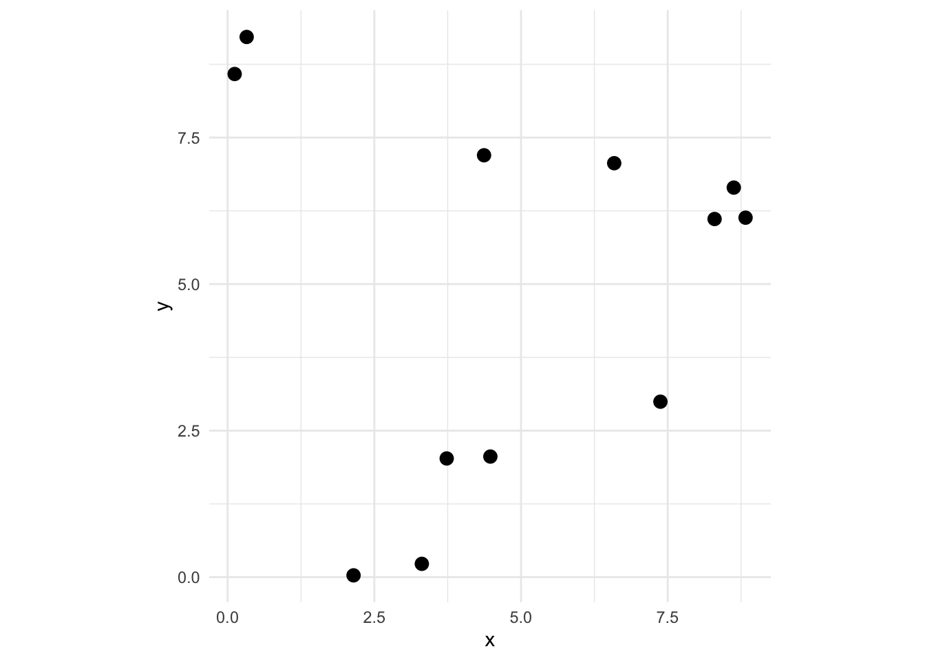
Ripley’s K at radius \(r\) is:
\[\hat{K}(r) = \frac{A}{n(n-1)} \sum_{i \neq j} I(d_{ij} \leq r)\]
Read it out loud: for each pair of distinct points \(i\) and \(j\), count whether they’re within distance \(r\) of each other. Sum those up, then scale by the area divided by \(n(n-1)\). That’s it.
So the first thing we need is all the pairwise distances. Build the distance matrix, then pull out every \(d_{ij}\) where \(i \neq j\). That means both the upper and lower triangles.
Dmat <- as.matrix(dist(cbind(x, y)))
Dmat
1 2 3 4 5 6 7 8
1 0.000000 2.222417 5.7901007 7.580887 4.144280 2.0801135 6.6235779 5.4316749
2 2.222417 0.000000 5.2117354 7.050732 5.168086 4.2919248 4.5209404 5.1412341
3 5.790101 5.211735 0.0000000 1.847110 3.768878 6.7301604 7.9582213 0.7447778
4 7.580887 7.050732 1.8471100 0.000000 4.918004 8.3349101 9.4716546 2.1712989
5 4.144280 5.168086 3.7688780 4.918004 0.000000 3.8606926 9.4041687 3.0456167
6 2.080113 4.291925 6.7301604 8.334910 3.860693 0.0000000 8.6903792 6.1860462
7 6.623578 4.520940 7.9582213 9.471655 9.404169 8.6903792 0.0000000 8.2759710
8 5.431675 5.141234 0.7447778 2.171299 3.045617 6.1860462 8.2759710 0.0000000
9 1.957775 4.076644 6.1263306 7.713813 3.250424 0.6280597 8.5577818 5.5701207
10 8.317389 7.504109 2.5490305 1.180277 6.010897 9.2606814 9.3641700 3.0895000
11 2.424025 4.582457 6.5435977 8.082010 3.458473 0.5511205 9.0441544 5.9603369
12 6.644890 4.470439 7.4887703 8.945120 9.159779 8.7243085 0.6641843 7.8476637
9 10 11 12
1 1.9577745 8.317389 2.4240253 6.6448902
2 4.0766438 7.504109 4.5824565 4.4704389
3 6.1263306 2.549030 6.5435977 7.4887703
4 7.7138132 1.180277 8.0820097 8.9451198
5 3.2504243 6.010897 3.4584727 9.1597788
6 0.6280597 9.260681 0.5511205 8.7243085
7 8.5577818 9.364170 9.0441544 0.6641843
8 5.5701207 3.089500 5.9603369 7.8476637
9 0.0000000 8.649843 0.5285956 8.5448918
10 8.6498428 0.000000 9.0484201 8.7901153
11 0.5285956 9.048420 0.0000000 9.0454998
12 8.5448918 8.790115 9.0454998 0.0000000Dvec <- c(Dmat[upper.tri(Dmat)], Dmat[lower.tri(Dmat)])
Dvec [1] 2.2224172 5.7901007 5.2117354 7.5808871 7.0507318 1.8471100 4.1442796
[8] 5.1680862 3.7688780 4.9180036 2.0801135 4.2919248 6.7301604 8.3349101
[15] 3.8606926 6.6235779 4.5209404 7.9582213 9.4716546 9.4041687 8.6903792
[22] 5.4316749 5.1412341 0.7447778 2.1712989 3.0456167 6.1860462 8.2759710
[29] 1.9577745 4.0766438 6.1263306 7.7138132 3.2504243 0.6280597 8.5577818
[36] 5.5701207 8.3173887 7.5041090 2.5490305 1.1802771 6.0108972 9.2606814
[43] 9.3641700 3.0895000 8.6498428 2.4240253 4.5824565 6.5435977 8.0820097
[50] 3.4584727 0.5511205 9.0441544 5.9603369 0.5285956 9.0484201 6.6448902
[57] 4.4704389 7.4887703 8.9451198 9.1597788 8.7243085 0.6641843 7.8476637
[64] 8.5448918 8.7901153 9.0454998 2.2224172 5.7901007 7.5808871 4.1442796
[71] 2.0801135 6.6235779 5.4316749 1.9577745 8.3173887 2.4240253 6.6448902
[78] 5.2117354 7.0507318 5.1680862 4.2919248 4.5209404 5.1412341 4.0766438
[85] 7.5041090 4.5824565 4.4704389 1.8471100 3.7688780 6.7301604 7.9582213
[92] 0.7447778 6.1263306 2.5490305 6.5435977 7.4887703 4.9180036 8.3349101
[99] 9.4716546 2.1712989 7.7138132 1.1802771 8.0820097 8.9451198 3.8606926
[106] 9.4041687 3.0456167 3.2504243 6.0108972 3.4584727 9.1597788 8.6903792
[113] 6.1860462 0.6280597 9.2606814 0.5511205 8.7243085 8.2759710 8.5577818
[120] 9.3641700 9.0441544 0.6641843 5.5701207 3.0895000 5.9603369 7.8476637
[127] 8.6498428 0.5285956 8.5448918 9.0484201 8.7901153 9.0454998Why both triangles? Because \(d_{ij}\) and \(d_{ji}\) are the same distance, but the formula counts each ordered pair separately. Including both is what makes the denominator \(n(n-1)\) rather than \(n(n-1)/2\).
Now set a sequence of radii to evaluate K at, and loop.
r <- seq(0, 2.5, by = 0.1)

Kr <- numeric(length(r))
for (i in seq_along(r)) {
  Kr[i] <- (area / (n * (n - 1))) * sum(Dvec <= r[i])
}
Plot it against the theoretical K under complete spatial randomness, which is \(\pi r^2\).
kCurves <- tibble(
  r = r,
  Observed = Kr,
  `Theoretical (CSR)` = pi * r^2
) %>%
  pivot_longer(-r, names_to = "series", values_to = "K")

ggplot(kCurves, aes(x = r, y = K, color = series, linetype = series)) +
  geom_line(linewidth = 1) +
  scale_color_manual(
    values = c("Observed" = "#D55E00", "Theoretical (CSR)" = "grey40")
  ) +
  scale_linetype_manual(
    values = c("Observed" = "solid", "Theoretical (CSR)" = "dashed")
  ) +
  labs(y = "K(r)", x = "r", color = NULL, linetype = NULL) +
  theme_minimal() +
  theme(legend.position = "top")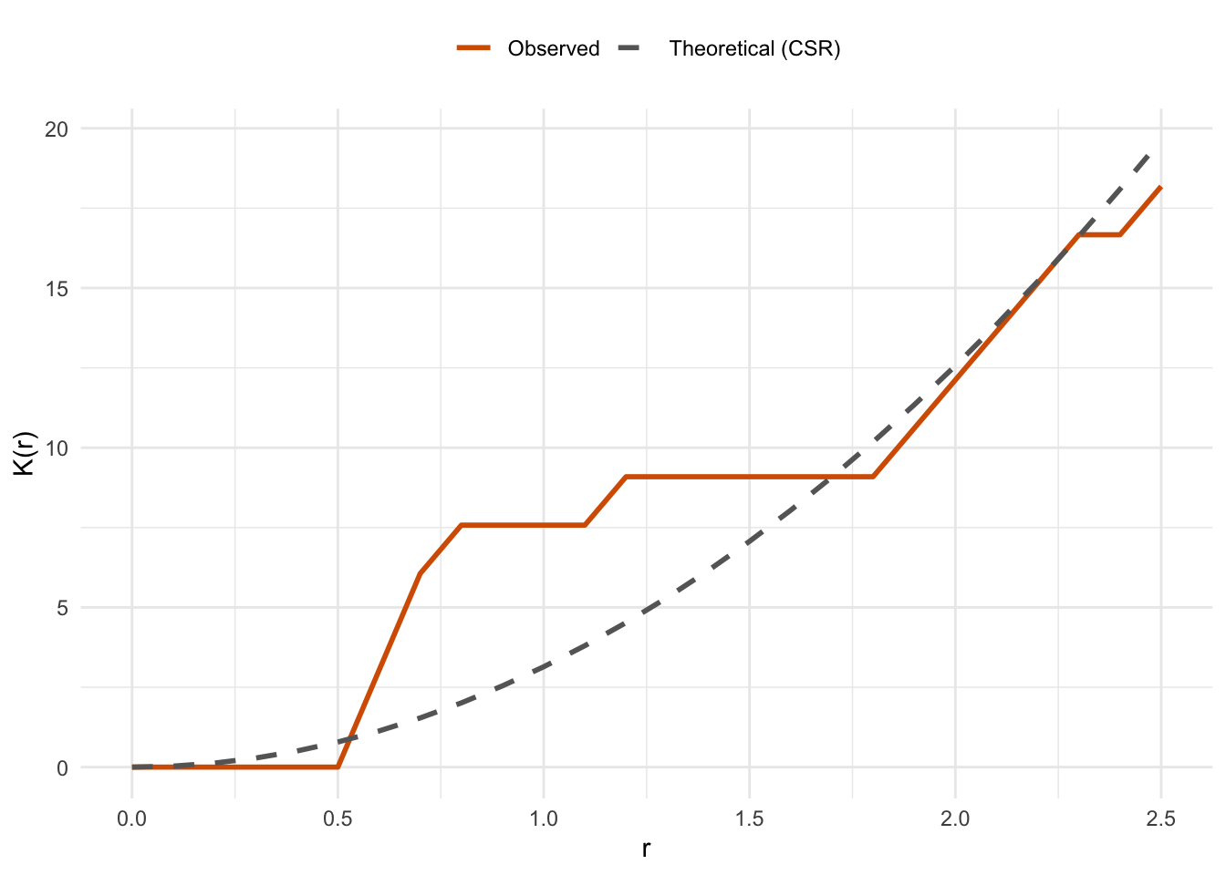
When the observed curve runs above the CSR reference, points are more clustered than random at that scale. Below it, they’re more dispersed. Random points should track the reference line with some noise.
Kest()Now verify the hand calculation against spatstat. Convert to a ppp object with the same window, pass the same radii, and use correction = "none" to match the uncorrected version we computed.
xy <- as.ppp(cbind(x, y), W = c(0, 10, 0, 10))
xyK <- Kest(xy, r = r, correction = "none")
Overlay the spatstat result on the plot. If everything is right, it should land exactly on our observed curve.
ggplot() +
  geom_line(
    data = kCurves, aes(x = r, y = K, color = series, linetype = series),
    linewidth = 1
  ) +
  geom_point(
    data = xyK, aes(x = r, y = un, shape = "Kest()"),
    size = 1.8
  ) +
  scale_color_manual(
    values = c("Observed" = "#D55E00", "Theoretical (CSR)" = "grey40")
  ) +
  scale_linetype_manual(
    values = c("Observed" = "solid", "Theoretical (CSR)" = "dashed")
  ) +
  scale_shape_manual(values = c("Kest()" = 1)) +
  labs(y = "K(r)", x = "r", color = NULL, linetype = NULL, shape = NULL) +
  theme_minimal() +
  theme(legend.position = "top")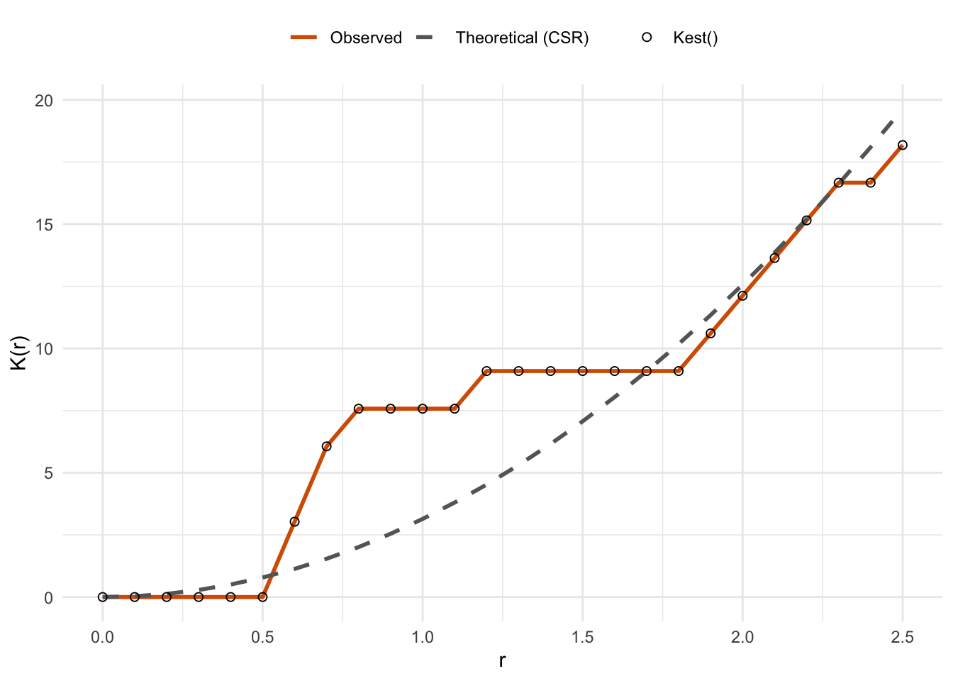
The open circles from Kest() sit right on top of our hand-computed curve. That’s reassuring. It also means that when you use Kest() in the main chapter, you know exactly what it’s computing.
One thing Kest() does that we didn’t do here: edge corrections. Points near the boundary of the study area have fewer neighbors within radius \(r\) than interior points do, simply because part of the circle falls outside the window. Without a correction, K is systematically underestimated at larger radii. The correction argument in Kest() handles this. The default is "isotropic", which is appropriate for most cases. Now that you understand the core calculation, the correction is a detail and not a mystery.