Code
library(spatialreg)
library(spdep)
library(sf)
library(tidyverse)The GLS chapter gave us one tool for handling spatially autocorrelated residuals: specify the correlation structure with a variogram and let GLS down-weight correlated observations. That works well. But there is a whole family of spatial regression models that take a different approach, and understanding them will round out your toolkit and sharpen your thinking about what spatial structure in a regression actually means.
GLS models the error correlation structure using a variogram, a continuous function of distance. The SAR (Simultaneous AutoRegressive) family instead uses an explicit spatial weights matrix: the same neighbor structure you built for Moran’s I and LISA. Two SAR models matter most for applied environmental work. The spatial error model says that the errors (the stuff your predictors don’t explain) are spatially correlated via a neighbor process. The spatial lag model says something more provocative: that the response variable at each location is directly influenced by the response at neighboring locations. These two models answer different questions, and it matters which one you fit.
This module follows directly from the Regression: GLS chapter and assumes you are comfortable with the OLS-to-GLS workflow there. The spatial weights machinery is the same as in the LISA chapter.
library(spatialreg)
library(spdep)
library(sf)
library(tidyverse)spatialreg (Bivand et al. 2021) carries the main functions for fitting SAR models. It was spun off from spdep (Bivand 2026) a few years ago, which means older code you find online might load these functions from spdep directly. If you see spdep::lagsarlm() in old tutorials, that is the same function. Load spatialreg explicitly. We also use sf (Pebesma 2026) for spatial data structures and tidyverse (Wickham 2023) for data wrangling.
We have two models that fall under the SAR umbrella. The spatial error model treats space as a nuisance: your predictors miss some spatially structured signal, so the leftover errors are correlated across neighbors. The spatial lag model treats space as part of the mechanism: the response at one location is pulled toward the response at its neighbors, a spillover built into the process itself. We sketched both in the Big Idea. Now let’s write them down and see exactly what each claims, because each is a small modification of the regression you already know and picking the right one is the objective here.
The models below are written in matrix notation. Don’t let that throw you. It is the same regression you already know, just written for all the locations at once instead of one row at a time. If you want to see how the matrix form works from the ground up, the OLS algebra aside walks through it.
In what follows, \(\mathbf{y}\) is a vector of \(n\) response values (one per location), \(\mathbf{X}\) is the design matrix, \(\boldsymbol{\beta}\) is the vector of regression coefficients, and \(\mathbf{W}\) is the spatial weights matrix you already know from Moran’s I and LISA. The operation \(\mathbf{W}\mathbf{y}\) computes a weighted average of \(y\) at neighboring locations. That is the spatial lag.
You will also notice that the same Greek letters appear here with different meanings than they had in earlier chapters. In the kriging chapter, \(\lambda\) was the vector of interpolation weights. Here it is a scalar measuring how strongly errors are correlated across neighbors. In the GLS chapter, \(\rho\) appeared in the code as the parameter we used to generate autocorrelated errors. Here \(\rho\) is the spatial autoregression coefficient on the response itself. This is not a conspiracy. Notation is there to serve the math, not to rule it, and the same letters get recycled constantly across fields, papers, and packages. Treat each symbol as local to what you are reading. Notation getting re-purposed and changed is annoying but something we just have to get used to.
Spatial error model (SEM):
\[\mathbf{y} = \mathbf{X}\boldsymbol{\beta} + \mathbf{u}, \quad \mathbf{u} = \lambda \mathbf{W} \mathbf{u} + \boldsymbol{\varepsilon}\]
The residuals \(\mathbf{u}\) follow a spatial autoregressive process. A residual at location \(i\) is a function of the residuals at its neighbors (via \(\lambda \mathbf{W}\)) plus independent noise \(\boldsymbol{\varepsilon}\). The coefficient \(\lambda\) (lambda) captures how strongly residuals are autocorrelated across neighbors. The coefficients \(\boldsymbol{\beta}\) have the same interpretation as in OLS: a one-unit increase in \(x\) is associated with a \(\beta_1\) change in \(y\), on average, holding everything else constant.
Ecologically, the SEM is the right choice when space is a nuisance. Your predictors don’t capture all the spatial structure in \(y\), so the leftovers are autocorrelated. Classic example: you’re modeling tree growth as a function of soil nitrogen, but soil moisture, microclimate, and a dozen other unmeasured things also drive growth and are themselves spatially structured. The SEM absorbs that shared unmeasured spatial structure into the error term and gives you clean, valid inference on the nitrogen-growth relationship.
Spatial lag model (SLM):
\[\mathbf{y} = \rho \mathbf{W} \mathbf{y} + \mathbf{X}\boldsymbol{\beta} + \boldsymbol{\varepsilon}\]
Now the response variable \(\mathbf{y}\) at each location appears on both sides of the equation. It is a function of \(\mathbf{W}\mathbf{y}\) (the weighted average of \(y\) at neighboring locations) plus your predictors \(\mathbf{X}\) and independent noise \(\boldsymbol{\varepsilon}\). The coefficient \(\rho\) (rho) is a scalar that captures how strongly \(y\) at one location is pulled toward \(y\) at its neighbors.
This is a fundamentally different claim from the SEM. The SLM says there is a spatial spillover process: \(y\) at one location influences \(y\) at neighboring locations. Classic examples are disease spread (infection rate in one area influences neighboring areas), invasive species dispersal (abundance at one site drives colonization of nearby sites), or any system where diffusion, movement, or contagion is part of the process. If the biology or ecology predicts that kind of mechanism, the lag model is the one to reach for.
One important caution: the \(\boldsymbol{\beta}\) coefficients from the SLM are not total marginal effects. More on this below.
There is a diagnostic test for choosing the appropriate model. The Rao score tests in spdep::lm.RStests() take an OLS fit and a weights matrix and test for evidence of spatial error vs spatial lag structure in the residuals. You get five test statistics from test = "all":
The names look like alphabet soup, but they decode cleanly. RS is Rao’s Score, the statistic that econometrics calls the Lagrange Multiplier. Same test, two names, which is why the function is lm.RStests, why older tutorials call these the LM tests, and why this section is headed that way too. The suffix says what is being tested: err for error dependence, lag for lag dependence. The adj prefix means adjusted, or robust: adjusted to stay valid when the other kind of dependence is also present, so adjRSerr tests for error while shrugging off any lag structure and adjRSlag does the reverse. SARMA stands for Spatial AutoRegressive Moving Average. A lag term is the autoregressive part and a spatially correlated error behaves like the moving-average part, so a process carrying both is a spatial ARMA, and the SARMA statistic is the joint test for whether either one is there.
The decision tree is simple. If only one of RSerr or RSlag is significant, fit that model. If both are significant, look at the robust tests and fit whichever of adjRSerr or adjRSlag is more significant. If neither is significant, OLS is fine.
We will build two simulated datasets, both in the spirit of the GLS chapter: a response \(y\) that is a function of a single predictor \(x\). What changes between them is how space gets in. In this first one the errors are spatially autocorrelated, so the spatial error model is the right answer. In the second, \(y\) itself spills over to neighbors, and the lag model is the right answer. Building the data ourselves means we know the truth and can check whether the workflow recovers it.
Start with the error process. Run the LM tests, confirm they point to the error model, then fit both models and see what each gives us.
n <- 75
easting <- runif(n, 0, 100)
northing <- runif(n, 0, 100)
points <- cbind(easting, northing)

# Build spatially autocorrelated errors via a SAR process
dnb <- dnearneigh(x = points, d1 = 0, d2 = 150)
dsts <- nbdists(nb = dnb, coords = points)
p <- 2.25
idw <- lapply(dsts, function(x) x^-p)
wList <- nb2listw(neighbours = dnb, glist = idw, style = "W")

inv <- spatialreg::invIrW(x = wList, rho = 0.75)
epsilon <- inv %*% rnorm(n)
epsilon <- scale(epsilon[, 1])[, 1]

# Response variable: y is a function of x plus autocorrelated noise
x <- rnorm(n)
B0 <- 3
B1 <- 0.5
y <- B0 + B1 * x + epsilon

dat <- data.frame(easting, northing, y, x)
We also need a k-nearest-neighbor weights matrix for the SAR models. Same approach as the LISA chapter.
nbK8 <- knn2nb(knearneigh(points, k = 8))
W <- nb2listw(nbK8, style = "W")Start with OLS.
ols <- lm(y ~ x, data = dat)
dat$olsResids <- residuals(ols)
moran.test(dat$olsResids, W)
    Moran I test under randomisation

data:  dat$olsResids
weights: W

Moran I statistic standard deviate = 7.0468, p-value = 9.152e-13
alternative hypothesis: greater
sample estimates:
Moran I statistic       Expectation          Variance
      0.343949179      -0.013513514       0.002573207
Moran’s I on the OLS residuals comes back at 0.34 with a vanishingly small p-value. We built the problem in, and there it is. Run the LM tests.
lm.RStests(ols, listw = W, test = "all")
    Rao's score (a.k.a Lagrange multiplier) diagnostics for spatial
    dependence

data:
model: lm(formula = y ~ x, data = dat)
test weights: W

RSerr = 39.288, df = 1, p-value = 3.657e-10


    Rao's score (a.k.a Lagrange multiplier) diagnostics for spatial
    dependence

data:
model: lm(formula = y ~ x, data = dat)
test weights: W

RSlag = 31.251, df = 1, p-value = 2.267e-08


    Rao's score (a.k.a Lagrange multiplier) diagnostics for spatial
    dependence

data:
model: lm(formula = y ~ x, data = dat)
test weights: W

adjRSerr = 8.5111, df = 1, p-value = 0.00353


    Rao's score (a.k.a Lagrange multiplier) diagnostics for spatial
    dependence

data:
model: lm(formula = y ~ x, data = dat)
test weights: W

adjRSlag = 0.47438, df = 1, p-value = 0.491


    Rao's score (a.k.a Lagrange multiplier) diagnostics for spatial
    dependence

data:
model: lm(formula = y ~ x, data = dat)
test weights: W

SARMA = 39.763, df = 2, p-value = 2.321e-09
Both RSerr (p = 3.7e-10) and RSlag (p = 2.3e-8) are significant. That is normal. A spatial error process produces apparent lag structure because the autocorrelated errors bleed into the response. So look at the robust tests. adjRSerr stays significant (p = 0.004) while adjRSlag does not (p = 0.49). That points to the error model, which is the right answer, since that is how we built the data.
semFit <- errorsarlm(y ~ x, data = dat, listw = W)
summary(semFit)
Call:errorsarlm(formula = y ~ x, data = dat, listw = W)

Residuals:
      Min        1Q    Median        3Q       Max
-1.832670 -0.516352 -0.011576  0.503105  2.692372

Type: error
Coefficients: (asymptotic standard errors)
            Estimate Std. Error z value  Pr(>|z|)
(Intercept) 3.096759   0.336247  9.2098 < 2.2e-16
x           0.482327   0.086319  5.5877 2.301e-08

Lambda: 0.72049, LR test value: 23.41, p-value: 1.3092e-06
Asymptotic standard error: 0.10165
    z-value: 7.0877, p-value: 1.3636e-12
Wald statistic: 50.235, p-value: 1.3636e-12

Log likelihood: -94.04644 for error model
ML residual variance (sigma squared): 0.66157, (sigma: 0.81337)
Number of observations: 75
Number of parameters estimated: 4
AIC: 196.09, (AIC for lm: 217.5)
The coefficient table gives \(\hat\beta_0 = 3.10\) and \(\hat\beta_1 = 0.48\), interpreted exactly like OLS coefficients and sitting right on the values we built in (\(\beta_0 = 3\), \(\beta_1 = 0.5\)). The extra parameter is \(\lambda = 0.72\), the spatial autocorrelation in the errors. A value near 1 means strong spatial error dependence; near 0 means the error model adds little over OLS. We generated the errors with \(\rho = 0.75\), so the model is recovering the dependence we put in.
Check the residuals.
dat$semResids <- residuals(semFit)
moran.test(dat$semResids, W)
    Moran I test under randomisation

data:  dat$semResids
weights: W

Moran I statistic standard deviate = 1.0261, p-value = 0.1524
alternative hypothesis: greater
sample estimates:
Moran I statistic       Expectation          Variance
      0.038829368      -0.013513514       0.002601947
Moran’s I on the SEM residuals falls to 0.04 (p = 0.15). The spatial structure has been pulled into \(\lambda\) and what is left looks like independent noise.
For comparison, fit the lag model on the same data.
slmFit <- lagsarlm(y ~ x, data = dat, listw = W)
summary(slmFit)
Call:lagsarlm(formula = y ~ x, data = dat, listw = W)

Residuals:
      Min        1Q    Median        3Q       Max
-2.068155 -0.557181  0.051375  0.542870  2.708741

Type: lag
Coefficients: (asymptotic standard errors)
            Estimate Std. Error z value  Pr(>|z|)
(Intercept)  1.14051    0.38178  2.9874  0.002814
x            0.43158    0.09069  4.7589 1.947e-06

Rho: 0.62184, LR test value: 18.187, p-value: 2.0028e-05
Asymptotic standard error: 0.11873
    z-value: 5.2375, p-value: 1.6277e-07
Wald statistic: 27.431, p-value: 1.6277e-07

Log likelihood: -96.65795 for lag model
ML residual variance (sigma squared): 0.72882, (sigma: 0.85371)
Number of observations: 75
Number of parameters estimated: 4
AIC: 201.32, (AIC for lm: 217.5)
LM test for residual autocorrelation
test value: 10.136, p-value: 0.0014539
The lag model estimates \(\rho = 0.62\), the spatial autoregression of the response, also significant. Because the data were generated under an error process, this is the wrong model. The two models are related, so it fits, but the LM tests already pointed us elsewhere and the AIC says so. Take a look:
AIC(semFit, slmFit) df AIC
semFit 4 196.0929
slmFit 4 201.3159The SEM wins. LM tests first, then model fitting, then AIC as a sanity check. Internalize that order.
That is the error model working on data we knew was an error process. Now build the other kind.
This time we build a spillover process. We generate \(y\) from the lag model’s reduced form, \(\mathbf{y} = (\mathbf{I} - \rho\mathbf{W})^{-1}(\mathbf{X}\boldsymbol{\beta} + \boldsymbol{\varepsilon})\), with \(\rho = 0.6\). Don’t worry about that formula yet. We unpack it in the next section. For now it is just the machinery that makes each location’s \(y\) depend on its neighbors’ \(y\). Same predictor \(x\), same true coefficients as before.
set.seed(2024)
n <- 75
easting <- runif(n, 0, 100)
northing <- runif(n, 0, 100)
points <- cbind(easting, northing)

nbK8 <- knn2nb(knearneigh(points, k = 8))
W <- nb2listw(nbK8, style = "W")

x <- rnorm(n)
B0 <- 3
B1 <- 0.5
rho <- 0.6

# Generate y from the lag reduced form
inv <- spatialreg::invIrW(W, rho = rho)
y <- as.numeric(inv %*% (B0 + B1 * x + rnorm(n)))

dat <- data.frame(easting, northing, y, x)Same opening moves as before, so we don’t have to linger. Reread above as needed. Let’s fit OLS, check the residuals, run the tests.
ols <- lm(y ~ x, data = dat)
dat$olsResids <- residuals(ols)
moran.test(dat$olsResids, W)
    Moran I test under randomisation

data:  dat$olsResids
weights: W

Moran I statistic standard deviate = 6.1474, p-value = 3.937e-10
alternative hypothesis: greater
sample estimates:
Moran I statistic       Expectation          Variance
      0.304877298      -0.013513514       0.002682463
Moran’s I shows that we have spatial structure, same as the first toy. The tests tell us what kind.
lm.RStests(ols, listw = W, test = "all")
    Rao's score (a.k.a Lagrange multiplier) diagnostics for spatial
    dependence

data:
model: lm(formula = y ~ x, data = dat)
test weights: W

RSerr = 30.365, df = 1, p-value = 3.58e-08


    Rao's score (a.k.a Lagrange multiplier) diagnostics for spatial
    dependence

data:
model: lm(formula = y ~ x, data = dat)
test weights: W

RSlag = 40.793, df = 1, p-value = 1.693e-10


    Rao's score (a.k.a Lagrange multiplier) diagnostics for spatial
    dependence

data:
model: lm(formula = y ~ x, data = dat)
test weights: W

adjRSerr = 0.21207, df = 1, p-value = 0.6451


    Rao's score (a.k.a Lagrange multiplier) diagnostics for spatial
    dependence

data:
model: lm(formula = y ~ x, data = dat)
test weights: W

adjRSlag = 10.64, df = 1, p-value = 0.001107


    Rao's score (a.k.a Lagrange multiplier) diagnostics for spatial
    dependence

data:
model: lm(formula = y ~ x, data = dat)
test weights: W

SARMA = 41.005, df = 2, p-value = 1.247e-09
Here is where this toy parts ways with the last one. Both RSerr and RSlag are significant again, but the robust tests now point the other way. adjRSlag is significant (p = 0.001) and adjRSerr is not (p = 0.65). Last time it was the reverse. The diagnostic is earning its keep: it can tell a lag process from an error process even though the raw tests look nearly identical in both.
Fit the lag model.
slmFit <- lagsarlm(y ~ x, data = dat, listw = W)
summary(slmFit)
Call:lagsarlm(formula = y ~ x, data = dat, listw = W)

Residuals:
      Min        1Q    Median        3Q       Max
-2.994524 -0.515842 -0.033154  0.706154  2.148501

Type: lag
Coefficients: (asymptotic standard errors)
            Estimate Std. Error z value  Pr(>|z|)
(Intercept)  3.75405    0.96314  3.8977 9.710e-05
x            0.79055    0.11715  6.7484 1.495e-11

Rho: 0.52863, LR test value: 19.876, p-value: 8.265e-06
Asymptotic standard error: 0.1193
    z-value: 4.4311, p-value: 9.3768e-06
Wald statistic: 19.634, p-value: 9.3768e-06

Log likelihood: -105.275 for lag model
ML residual variance (sigma squared): 0.93261, (sigma: 0.96572)
Number of observations: 75
Number of parameters estimated: 4
AIC: 218.55, (AIC for lm: 236.43)
LM test for residual autocorrelation
test value: 3.1924, p-value: 0.073982
\(\rho = 0.53\), highly significant and close to the 0.6 we built in. Check the residuals.
dat$slmResids <- residuals(slmFit)
moran.test(dat$slmResids, W)
    Moran I test under randomisation

data:  dat$slmResids
weights: W

Moran I statistic standard deviate = -0.91795, p-value = 0.8207
alternative hypothesis: greater
sample estimates:
Moran I statistic       Expectation          Variance
     -0.060755818      -0.013513514       0.002648666
Moran’s I drops to -0.06, nowhere near significant. The lag term has soaked up the spatial structure. AIC confirms the lag model over both OLS and the error model:
semFit <- errorsarlm(y ~ x, data = dat, listw = W)
AIC(ols, semFit, slmFit)
df AIC
ols 3 236.4256
semFit 4 222.2312
slmFit 4 218.5500The SLM wins, 218.6 against 222.2 for the SEM and 236.4 for OLS. LM tests, model fit, and AIC all agree this is a lag process.
Now the payoff, and the reason the lag model needs more care than the error model. In OLS or the SEM, \(\hat\beta_1\) is the whole story: a one-unit change in \(x\) moves \(y\) by \(\hat\beta_1\), full stop. Not so in the lag model. A change in \(x_i\) moves \(y_i\) directly, but that nudge to \(y_i\) then propagates to neighbors, because their \(y\) depends on \(y_i\) through the lag term, and those ripples feed back. The \(\hat\beta_1\) from lagsarlm is only the direct local piece, before the spatial propagation plays out. For the full marginal effect you compute impacts.
impacts(slmFit, listw = W, R = 500)Impact measures (lag, exact):
Direct Indirect Total
x dy/dx 0.8280221 0.8491201 1.677142The effect splits into direct (same location), indirect (spillover to neighbors), and total. Here the direct effect is 0.83, the indirect is 0.85, and the total is 1.68. The spillover is as large as the direct effect, so reporting the raw coefficient of 0.79 alone would understate the full effect by more than half. When you fit a lag model, the total impacts are what you report.
A caution to close the toy on. This decomposition means something here only because we know there is a spillover process; we built one. Run the same impacts() on the error toy from the previous section and it would report spillover too, except there it would be an artifact, the lag model inventing a mechanism that is not in the data. The lag model makes a more specific, more mechanistic claim than the error model, and the LM tests are what keep you on the right side of that line. Fit it when the diagnostics and the science both point to spillover, not just because the function returns a number.
Both the SEM and GLS attack the same problem: errors correlated across space rather than independent. And they are closer than they look. In the OLS algebra aside we wrote GLS as OLS reweighted by \(\boldsymbol{\Sigma}^{-1}\), where \(\boldsymbol{\Sigma}\) is the covariance matrix of the errors. The SEM is the same kind of model. It also assumes \(\mathbf{y} = \mathbf{X}\boldsymbol{\beta} + \mathbf{u}\) with a structured \(\boldsymbol{\Sigma}\). What differs is where \(\boldsymbol{\Sigma}\) comes from.
GLS builds \(\boldsymbol{\Sigma}\) from a variogram: a smooth function of distance with a range, a sill, and a nugget. You pick the shape of the distance decay and let the data fit its parameters. Every pair of points is correlated to a degree that depends only on how far apart they sit.
The SEM builds \(\boldsymbol{\Sigma}\) from the neighbor process instead. Start from its definition, \(\mathbf{u} = \lambda\mathbf{W}\mathbf{u} + \boldsymbol{\varepsilon}\), and solve for \(\mathbf{u}\):
\[(\mathbf{I} - \lambda\mathbf{W})\mathbf{u} = \boldsymbol{\varepsilon} \quad\Longrightarrow\quad \mathbf{u} = (\mathbf{I} - \lambda\mathbf{W})^{-1}\boldsymbol{\varepsilon}\]
Here \(\mathbf{I}\) is the identity matrix, the matrix version of the number 1: ones down the diagonal, zeros everywhere else, so \(\mathbf{I}\mathbf{u} = \mathbf{u}\). You met it in that same aside, where \(\boldsymbol{\Sigma} = \sigma^2\mathbf{I}\) was the independent-errors case that collapses GLS back to OLS. Here it lets us peel \(\mathbf{u}\) off onto one side. The payoff is that the SEM’s error covariance works out to
\[\boldsymbol{\Sigma} = \sigma^2\left[(\mathbf{I} - \lambda\mathbf{W})^T(\mathbf{I} - \lambda\mathbf{W})\right]^{-1}\]
One scalar \(\lambda\), plus the weights matrix \(\mathbf{W}\) you already built, generates the whole covariance. You never specify a distance-decay curve. It falls out of the graph.
That difference has a nice consequence. \(\mathbf{W}\) is sparse: it connects each point only to its handful of neighbors. But the inverse \((\mathbf{I} - \lambda\mathbf{W})^{-1}\) is dense. Inverting the matrix lets dependence leak past the immediate neighbors, so your neighbor’s neighbor is correlated with you too, just more weakly, and so on outward. A local rule produces global structure. That is what you want from a spatial process, and it is why the SEM can mimic a smooth distance decay without ever being told about distance.
So when do you reach for which? GLS tends to win when you have a clear distance-decay structure and enough data to fit a variogram cleanly. The SEM tends to win when your data are naturally defined by adjacency or neighborhood (watershed catchments, habitat patches, gridded climate data) and you want to lean on the weights matrix you already built for Moran’s I and LISA. For the error case they often give you nearly the same answer, so the choice comes down to which framing fits your data and which machinery you trust.
The lag model is the one with no GLS equivalent. GLS and the SEM both leave \(\mathbf{y} = \mathbf{X}\boldsymbol{\beta} + \mathbf{u}\) alone and work on the error term. The lag model puts \(\mathbf{W}\mathbf{y}\) on the right-hand side and models the response itself, the spillover story from the second toy. If the science predicts diffusion or contagion, that is the model for it, and GLS has nothing that does the same job.
Enough simulation. Here is the whole workflow on data we didn’t build, where we don’t know the answer going in.
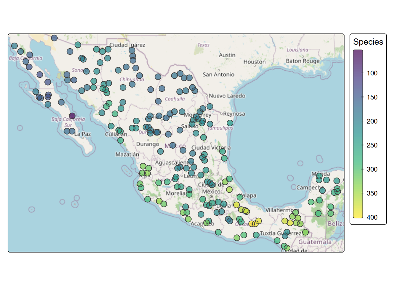
The birdRichnessMexico dataset has 200 point locations across Mexico with bird species richness (nSpecies) and six WorldClim bioclimatic variables extracted at each location. Maps use tmap (Tennekes 2018). Two predictors have strong ecological justification: mean annual precipitation (map) and temperature annual range (tempRange). Wetter areas support more species; thermally variable areas support fewer. That’s the energy-water hypothesis and Rapoport’s rule operating across the Mexican landscape.
library(tmap)
birdsSf <- readRDS("data/birdRichnessMexico.rds")
coordsBirds <- st_coordinates(birdsSf)

nbBirds <- knn2nb(knearneigh(coordsBirds, k = 8))
WBirds <- nb2listw(nbBirds, style = "W")
Map the richness surface first.
tmap_mode("plot")
tm_basemap("OpenStreetMap") +
  tm_shape(birdsSf) +
  tm_symbols(
    fill = "nSpecies",
    fill.scale = tm_scale_continuous(values = "viridis"),
    fill.legend = tm_legend(title = "Species"),
    fill_alpha = 0.7,
    size = 0.7
  )
olsBirds <- lm(nSpecies ~ map + tempRange, data = birdsSf)
summary(olsBirds)
Call:
lm(formula = nSpecies ~ map + tempRange, data = birdsSf)

Residuals:
     Min       1Q   Median       3Q      Max
-136.424  -13.629   -2.138   15.146   92.269

Coefficients:
              Estimate Std. Error t value Pr(>|t|)
(Intercept) 213.383856  15.079562  14.151  < 2e-16 ***
map           0.078438   0.004528  17.324  < 2e-16 ***
tempRange    -1.758331   0.473349  -3.715 0.000265 ***
---
Signif. codes:  0 '***' 0.001 '**' 0.01 '*' 0.05 '.' 0.1 ' ' 1

Residual standard error: 27.74 on 197 degrees of freedom
Multiple R-squared:  0.8009,    Adjusted R-squared:  0.7989
F-statistic: 396.3 on 2 and 197 DF,  p-value: < 2.2e-16
\(R^2\) of 0.80. Both predictors are significant with the expected signs. Now check the residuals.
That 0.80 is the most comforting number in this output and close to the least informative for what we need here. \(R^2\) measures how much variance the predictors soaked up, not whether the assumptions behind your standard errors hold, and spatial dependence lives entirely in that second thing. In a moment Moran’s I on these residuals comes back at 0.40: the model is missing a pile of spatial structure, and \(R^2\) had nothing to say about it. Notice too that when we fit the SEM, its summary won’t print an \(R^2\) at all. Once you fit by likelihood with a structured covariance, the tidy “variance explained” split stops being well defined, which the GLS chapter unpacks. From here on the residual diagnostics and AIC adjudicate the model, not \(R^2\).
birdsSf$ols_resids <- residuals(olsBirds)
moran.test(birdsSf$ols_resids, WBirds)
    Moran I test under randomisation

data:  birdsSf$ols_resids
weights: WBirds

Moran I statistic standard deviate = 12.42, p-value < 2.2e-16
alternative hypothesis: greater
sample estimates:
Moran I statistic       Expectation          Variance
      0.397871539      -0.005025126       0.001052372
Moran’s I is 0.40, strongly significant. The model explains 80% of the variance but the residuals carry substantial spatial signal. Map them to see where the model is over- and under-predicting.
tm_basemap("OpenStreetMap") +
  tm_shape(birdsSf) +
  tm_symbols(
    fill = "ols_resids",
    fill.scale = tm_scale_continuous(values = "-brewer.rd_bu", midpoint = 0),
    fill.legend = tm_legend(title = "Residual"),
    fill_alpha = 0.7,
    size = 0.7
  )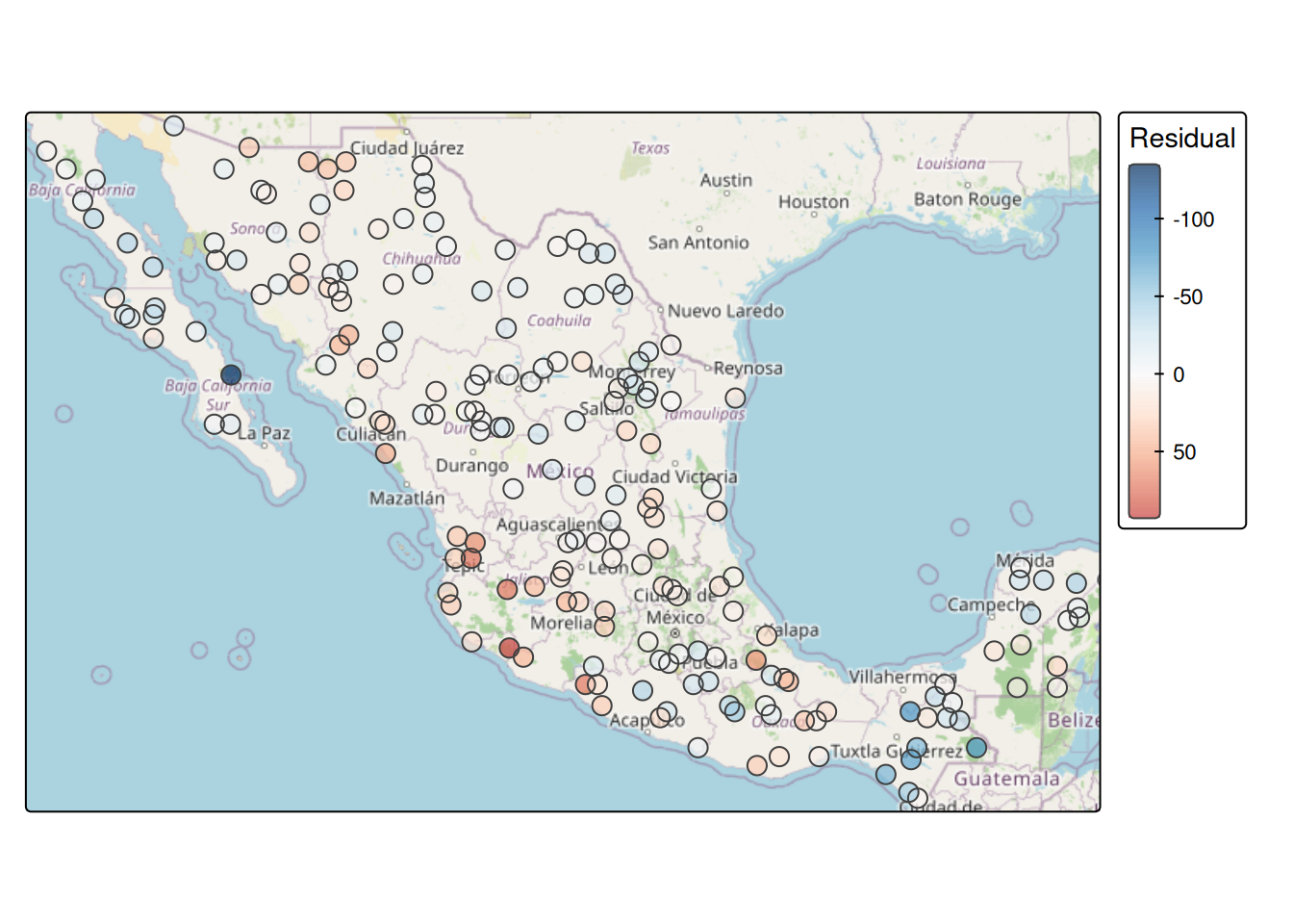
The pattern is not random. There are regions where richness is consistently higher than the climate model predicts and others where it’s consistently lower. That’s what Moran’s I is flagging, and the map shows you where.
lm.RStests(olsBirds, listw = WBirds, test = "all")
    Rao's score (a.k.a Lagrange multiplier) diagnostics for spatial
    dependence

data:
model: lm(formula = nSpecies ~ map + tempRange, data = birdsSf)
test weights: WBirds

RSerr = 140.81, df = 1, p-value < 2.2e-16


    Rao's score (a.k.a Lagrange multiplier) diagnostics for spatial
    dependence

data:
model: lm(formula = nSpecies ~ map + tempRange, data = birdsSf)
test weights: WBirds

RSlag = 33.448, df = 1, p-value = 7.321e-09


    Rao's score (a.k.a Lagrange multiplier) diagnostics for spatial
    dependence

data:
model: lm(formula = nSpecies ~ map + tempRange, data = birdsSf)
test weights: WBirds

adjRSerr = 107.73, df = 1, p-value < 2.2e-16


    Rao's score (a.k.a Lagrange multiplier) diagnostics for spatial
    dependence

data:
model: lm(formula = nSpecies ~ map + tempRange, data = birdsSf)
test weights: WBirds

adjRSlag = 0.37184, df = 1, p-value = 0.542


    Rao's score (a.k.a Lagrange multiplier) diagnostics for spatial
    dependence

data:
model: lm(formula = nSpecies ~ map + tempRange, data = birdsSf)
test weights: WBirds

SARMA = 141.18, df = 2, p-value < 2.2e-16
Same diagnostic as the toy example, same verdict. Both RSerr and RSlag fire. The robust adjRSerr is 108 and stays significant; adjRSlag is 0.37 and dies (p = 0.54). Error model.
semBirds <- errorsarlm(nSpecies ~ map + tempRange,
                       data = birdsSf, listw = WBirds
)
summary(semBirds)
Call:errorsarlm(formula = nSpecies ~ map + tempRange, data = birdsSf,
    listw = WBirds)

Residuals:
      Min        1Q    Median        3Q       Max
-133.6497  -12.8050    0.7134   11.8756   60.3406

Type: error
Coefficients: (asymptotic standard errors)
               Estimate  Std. Error z value  Pr(>|z|)
(Intercept) 245.0812381  20.1854257 12.1415 < 2.2e-16
map           0.0727603   0.0052084 13.9699 < 2.2e-16
tempRange    -2.7528488   0.6849927 -4.0188  5.85e-05

Lambda: 0.72462, LR test value: 74.723, p-value: < 2.22e-16
Asymptotic standard error: 0.059692
    z-value: 12.139, p-value: < 2.22e-16
Wald statistic: 147.36, p-value: < 2.22e-16

Log likelihood: -909.5156 for error model
ML residual variance (sigma squared): 478.86, (sigma: 21.883)
Number of observations: 200
Number of parameters estimated: 5
AIC: 1829, (AIC for lm: 1901.8)
Lambda is 0.72, highly significant. There is strong spatial autocorrelation in the errors above and beyond what precipitation and temperature range explain. Check the residuals.
birdsSf$sem_resids <- residuals(semBirds)
moran.test(birdsSf$sem_resids, WBirds)
    Moran I test under randomisation

data:  birdsSf$sem_resids
weights: WBirds

Moran I statistic standard deviate = 0.43109, p-value = 0.3332
alternative hypothesis: greater
sample estimates:
Moran I statistic       Expectation          Variance
      0.008848122      -0.005025126       0.001035655
Moran’s I drops to 0.009 (p = 0.33), indistinguishable from zero. The spatial structure has been absorbed into lambda. Compare AIC.
AIC(olsBirds, semBirds) df AIC
olsBirds 4 1901.754
semBirds 5 1829.031A drop of about 73 units. The error model is substantially better.
The coefficients shift after accounting for spatial error dependence. The effect of tempRange gets stronger: OLS estimated -1.76 species per degree of range; the SEM estimates -2.75. OLS was underestimating the temperature effect because spatially autocorrelated errors were confounding the estimate. The precipitation coefficient shifts less, from 0.078 to 0.073, which makes sense given how dominant that predictor is.
What does lambda = 0.72 mean ecologically? Precipitation and temperature range explain most of the richness gradient, but there’s substantial residual spatial structure they don’t capture. Some of it is almost certainly habitat heterogeneity: the Sierra Madre Occidental and Oriental are centers of endemism and provide topographic complexity that flat climate variables miss. Some may reflect historical biogeography. Proximity to the Neotropical source pool in southern Mexico leaves a signature that current climate alone doesn’t explain. The SEM doesn’t tell you what the missing variable is. It tells you that something spatially structured is out there and that ignoring it was biasing your inference.
GLS and SAR are corrections to the same problem: OLS residuals that carry spatial signal the model hasn’t explained. The error model and the lag model answer two different questions about that signal. Is space a nuisance, soaking up everything your predictors missed? Fit the error model, or GLS, and report clean coefficients. Or is space part of the mechanism, the response in one place driving the response next door? That is the lag model, and you owe the reader the impacts, not the raw coefficients.
Let the LM tests and the science decide, in that order. For most field-based environmental work the answer is the error case, and GLS is the workhorse: flexible, tied to the variogram, easy to read. Reach for SAR when a neighbor graph describes your data better than a distance decay, or when there is a credible spillover in the response itself. Think about how disease spreads, or how animal behavior in one patch influences the next. But for lead in floodplain soil, space is probably just a proxy for flood exposure. Use GLS and sleep well.
The Meuse River data contains several candidate predictors for soil lead contamination. river_dist_m is the distance from the river channel in meters and ffreq is a flooding frequency class (a factor with three levels: 1 = most frequent, 3 = least frequent). Both are plausible drivers of lead deposition: proximity to the channel means exposure to recent flood sediment, and flooding frequency determines how much sediment accumulates.
meuse2 <- readRDS("data/meuse2.Rds")
meuse.grid2 <- readRDS("data/meuse.grid2.Rds")
meuseSf <- st_as_sf(meuse2, coords = c("x", "y"), crs = 28992)
meuseSf$log_lead <- log(meuseSf$lead)
# get river distance and flooding frequency from the grid
covarsSf <- st_as_sf(meuse.grid2, coords = c("x", "y"), crs = 28992) %>%
  select(ffreq, river_dist_m)
meuseSf <- st_join(meuseSf, covarsSf, join = st_nearest_feature) %>%
  mutate(ffreq = factor(ffreq))
Build a k-nearest-neighbor weights matrix with \(k = 8\).
Fit OLS of log_lead ~ river_dist_m + ffreq. Interpret the coefficients. Do the signs make ecological sense? Run Moran’s I on the residuals.
Run the LM tests. Both RSerr and RSlag will be significant. Look at the robust tests to break the tie. Which model do they recommend?
Fit both the SEM and the SLM. Check the residuals of each using Moran’s I. One model cleans up the spatial structure; the other doesn’t. Which is which, and what does that tell you?
Compare AIC across OLS, SEM, and SLM. Does AIC agree with the LM tests?
Compare coefficients on river_dist_m and ffreq between OLS and the SEM. The point estimates shift and the standard errors change. What does the shift in standard errors tell you about what OLS was doing wrong?
Is the spatial error model or the spatial lag model more ecologically defensible for soil lead? What process would the lag model imply, and is that a plausible mechanism for how lead ends up in floodplain soil?
In the bird richness example, lambda = 0.72 after accounting for precipitation and temperature range. What do you think is driving the residual spatial structure? Name at least two candidate variables not in the model and explain why they might be spatially structured across Mexico.
Dormann et al. (2007) sections 3.3 and 3.4 cover spatial error models and related approaches. Bivand (2008) chapter 9 goes deep on the SAR model family and the spatialreg functions; it’s a technical chapter, but worth returning to once you’ve worked through the examples here.